Introduction

Ten years ago, Warren Buffet successfully bet that a low-cost Vanguard S&P 500 index fund would beat any managed fund portfolio picked by Protégé Partners.  Gary Antonacci's “Dual Momentum Investing: An Innovative Strategy for Higher Returns with Lower Risk” can be used to “tweak” Buffett’s simple money management approach by moving into cash when the S&P starts trending down, then moving back to the S&P fund when it trends up.  The trick, of course, is coming up with a proper trend function.  Jumping in and out of the market too frequently, even in ETFs, erodes returns, especially (apparently) if you are a guy. 

How Portfolio Visualizer calculates Relative, Absolute and Dual Momentum

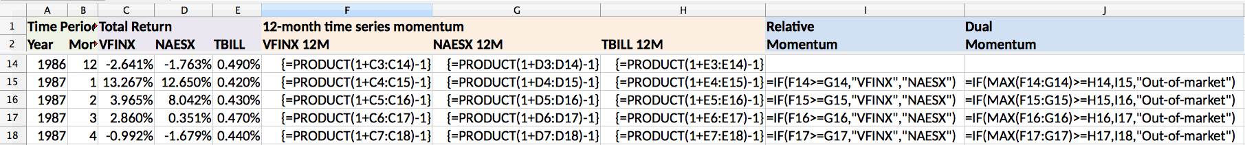
Below is how https://www.portfoliovisualizer.com/ calculates these quantities. (I want to give a shout out here to Tuomo Lampinen of Silicon Cloud Technologies, LLC, who answered all my questions about https://www.portfoliovisualizer.com/. As we will discover later, it is the (free) tool Al and James used to create the baseline examples I reference here.) VFINX is the main investment that (Ideally) you would be in all the time (Like the S&P 500). NAESX is the alternative (safe) investment that you use when VFINX is non performant. Finally, TBILLs is where you go when neither of these investments are performing. (Note that you could drop NAESX and just switch between VFINX and TBILLs.) Implicit in these calculations is the "lookback period" or "lag". This "lag" is the distance between cells in all the PRODUCT calculations. E.g. C3:C14 in cell F14. In excel, ranges are inclusive, so the lag is 14-3+1 = 12 months. In Python, ranges are exclusive and so would be expressed as [3:15] for 12 months.

Motivation

Al Zmyslowski (Docs: AAII-SV-CIMI1702.pdf) and Peter James Lingane (Docs: ThreeMomentumAlgorithms.pdf) presented Gary Antonacci's Dual Momentum Strategy at AAII-SV-CIMI on 20170202.  Al used portfoliovisualizer.com to do this.  Each ran a different portfolio, and each showed different performance which varied by timeframe.  I.e. the portfolio changed little before 2001 and flattened after 2015. This timeframe variance was also apparent at the 20170211 presentations at Cupertino AMC theaters by Gary Antonacci (Docs: 20170211Dual Momentum_Cupertino.pdf) and Peter James Lingane (Docs: 20170211AAII 2017_final.pdf). 

This lead me to wonder how the time behavior of this approach (and more generally, the market) changed over the years. That is, suppose you had a different 'lag' for each row in the above spreadsheet?'

Examining the market’s time behavior in the frequency domain

One approach to this question is to look at the frequency domain after the market has undergone a shock.  Pictures of the DJIA in October 1987 showed a an exponentially damped oscillation the day after the Market drop. I had hoped to see transients after Trump’s election.  Don Maurer was kind enough to provide minute data of this period.  Long story short, I was unable to find anything using FFTs.  However I have made the data available here (20170202FreqAnal).

Reproducing Portfolio Visualizer’s dual Momentum approach in pandas

Another approach is to work in the time domain.  Here, I first ran Al Zmyslowski’s and Peter Lingane’s 20170202 AAII-SV-CIMI Dual Momentum portfolio in https://www.portfoliovisualizer.com/ and then compared the results to a pandas implementation of Dual Momemtum.

It is worthwhile reviewing this effort, since my original assumptions about how to construct the model were wrong at practically every point.  To review my mistakes:

• TBill Rate Source - Not any TBill rate will do.  I started out with “SPDR Blmbg Barclays 1-3 Mth T-Bill ETF (BIL)”, but it did not go back far enough in time.  Tuomo suggested looking at the federal reserve and Farma French Data.  The sources I used are described on the Documentation page here (20170318createHistoryFiles).  As you will see later however, at the end of the day, the 3mo Tbill Rates seem to provide the best results. 
• Price Quote Source - Not any Price Quote source will do.  Yahoo (my source) differed from Portfolio visualizer in 3/384 quotes on the days listed below
• df.loc['1986-12-01','VFINX1']= -0.02641   ########################### I have -0.0987878061893
• df.loc['1986-10-01','NAESX1']=  0.03935   ########################### I have -0.104985
• df.loc['1987-12-01','NAESX1']=  0.11958   ########################### I have -0.00720177
• Return Calculation - The 20170211 presentation calculated return by division.  E.g. for 12 month return, it divided the current month’s stock price by its price 12 months ago.  Portfolio visualizer compounds the one month return.  This spot where this matters is the Farma French TBill Calculation, where F-F_Research_Data_Factors’ RF column needs to be compounded.
• Significance (Precision) - One thing to note in the above spreadsheet is that column E "TBILL", which comes from Farma French, has only 2 significant digits. That means that numbers in the thousanths place and beyond are insignificant. So although continuous compounding generates a bucketload of digits, only those above the thousanths place matter. This is reflected in fact that my python code differed from Portfolio visualizer in 3/384 calculations in the 3rd decimal place on the days listed below.
• # 0.097838024 0.0978231319 in VFINXlag NAESXlag
• df.loc['1992-11-02','DM'] = 'NAESXlag'  ########################### I have VFINXlag
• # 0.0552612318 0.0565098256 in NAESXlag FGOVXlag
• df.loc['2001-06-01','DM'] = 'NAESXlag'  ########################### I have FGOVXlag
• # 0.1564317439 0.1563179165 in VFINXlag NAESXlag
• df.loc['2007-01-03','DM'] = 'NAESXlag'  ########################### I have VFINXlag

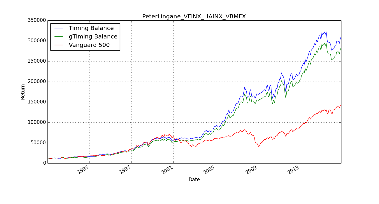
(20170324reproducePortfolioVisualizer) shows the effects of a corrected model (Al Zmyslowski’s) and an uncorrected model (Peter James Lingane). Peter's corrected and uncorrected model is shown below.'

Pandas “Dual Momentum” Algorithm’s sensitivity to lags and TBill Rates.

Despite the issues noted above, we use Yahoo quotes in the section (since we have no access to anything else).  Our version of Dual Momentum is passed a list of:

• portfolios - We limit ourselves to Als’ and James’ here.  However James’ performs best (VFINX,HAINX,VBMFX)
• TBill Rates - We use all rates recommended by Tuomo Lampinen.  However the Federal Reserve Board 3mo rate performs best. Don Maurer commented "In any case, the choice of which measure of risk free returns is used to make a decision of whether to be in or out of equities is somewhat arbitrary. A system should be “robust” to slight variations in that choice, otherwise, one choice may have just been lucky for that particular set of data. You’d hope that a slight dithering of the risk free data along the way wouldn’t make any big changes in the results – along the lines of how I used synthetic ECs to test price oriented timers. Therefore maybe we should dither the RF data returns and run 1000+ trials with different dithering of the returns and get a distribution of the results – again hoping they stay closely clustered like some but not all of the timers did." Unless my code is broken, there seem to be significant differences in Risk Free Rates. (See here) Using Don's (usually quite good) logic, this implies that the system is -not- robust and we have been lucky with the data we chose.
• Constant lags - We limited ourselves to all the lags listed in portfolioVisualizer. E.g. [1, 2, 3, 4, 5, 6, 7, 8, 9, 10, 11, 12, 15, 18, 21, 24, 27, 30, 33, 36] months lookback for all 384 time points. Interestingly, 21 month lookback gave about the same results as 12 month lookback in Lingane's portfolio for the majority of its lifetime, but performed worse after the 2007 crash and better over the last several years.

• or Variable lags - In addition, we created lag structures that steadily in/decrease over the span of 32 years from 8 to 24 months and 21 to 36 months. E.g. in python, 'lag8-23' is flatten([[z]*24 for z in range(8,24)]) # [24 eights, 24 nines... 24 twentythrees] This particular structure worked the best. It used 8 month lookback for each of the first 24 months, 9 month lookback for each of the next 24 months and increases up to 24 month lookback for each of the final 24 months. As Ken Keller has pointed out, the next step here is to use a learner to fill in each of the 384 time slots. Below is the summary of a number of runs. 20170327backtestLags shows more.

Summary

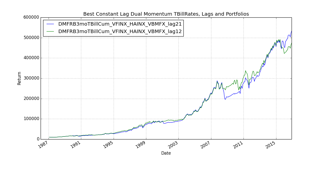
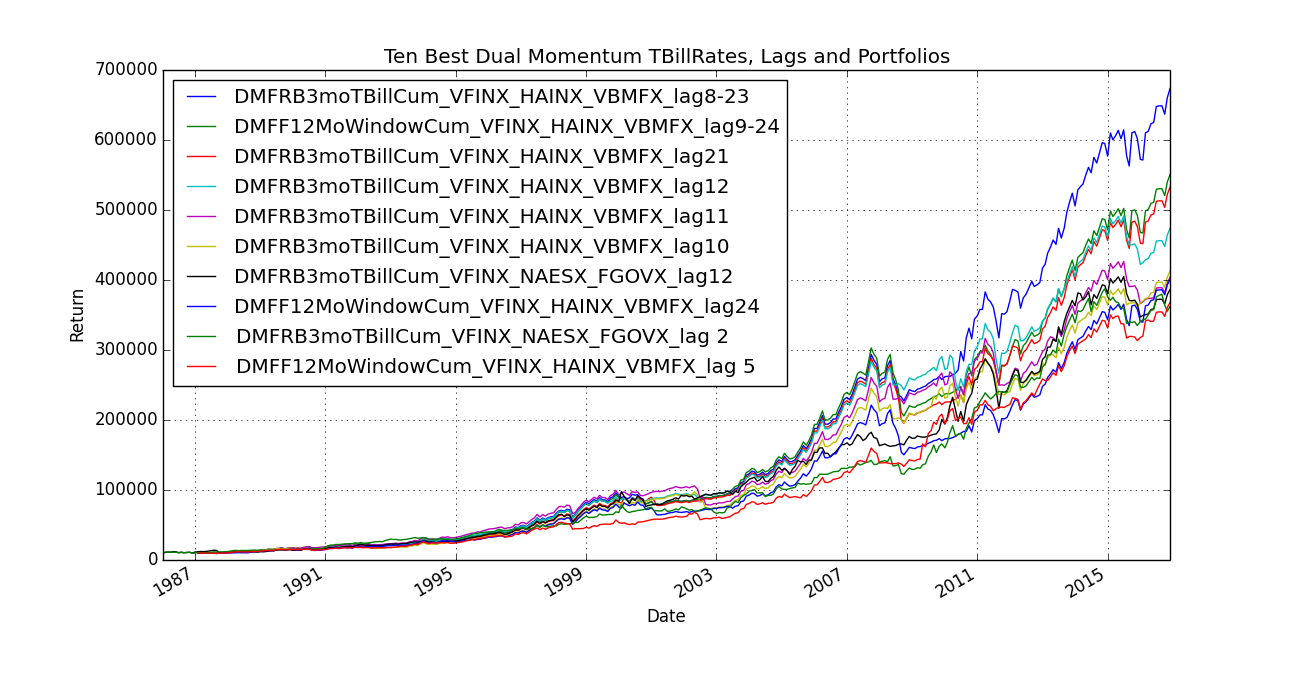
The basic idea I had was that things are moving faster and faster. As such, I guessed that one needed to adjust one's portfolio with shorter and shorter intervals. So if the 80's were the decade where one could check returns every 12 months, then the 2010's are the decade where you need to shorten the interval to checking every 6 months. (So I thought) So, nice theory, but actually the -reverse- gave better results: i.e. instead of a 23 month interval moving to an 8 month interval over time, the 8 month interval moving to a 23 month interval gave better results. The most enlightening chart to me is "Best Constant Lag Dual Momentum TBillRates, Lags and Portfolios". What's happening here is that during the crash, it made sense to move fast (12 month lag does better). But when things are going reasonably smoothly, it makes sense to hold on a little longer. (21 month lag is better). Crashes are easy to detect. Now all I need is a "reasonably smoothly" detector.

Docs lists all references.